Understanding Word2Vec and Doc2Vec
Word embeddings are a type of word representation which stores the contextual information in a low-dimensional vector. This approach gained extreme popularity with the introduction of Word2Vec in 2013, a groups of models to learn the word embeddings in a computationally efficient way. And Doc2Vec can be seen an extension of Word2Vec whose goal is to create a representational vector of a document.
Word2Vec and Doc2Vec are implemented in several packages/libraries. A python package called gensim implemented both Word2Vec and Doc2Vec. Google’s machine learning library tensorflow provides Word2Vec functionality. In addition, spark’s MLlib library also implements Word2Vec.
All of the Word2Vec and Doc2Vec packages/libraries above are out-of-the-box and ready to use. However, understanding the underlying theories and details behind the code will give us a better and clearer look of how to think about word embeddings. Also, it will help us better tune the model’s hyper-parameters if we know how they really work.
Word2Vec
Two most popular algorithms to create Word2Vec representations are Skip-Gram model and Continuous Bag-of-Words model (CBOW). Let’s get to the details of these two algorithms.
To give you an insight into what Word2Vec is doing, let’s first talk about it in an abstract way. Word2Vec uses a simple neural network with a single hidden layer to learn the weights. Different from most other machine learning models, we are not interested in the predictions this neural network could make. Instead, we only care about the weights of the hidden layer, since these weights are actually the word embeddings/vectors we are about to learn.
Skip-Gram
For the Skip-Gram model, the task of the simple neural network is: Given an input word in a sentence, the network will predict how likely it is for each word in the vocabulary being that input word’s nearby word.
The training examples to the neural network are word pairs which consist of the input word and its nearby words. For example, consider the sentence “He says make America great again.” and a window size of 2. The training examples are:
| Sentence | Training examples |
|---|---|
| He says make America great again. | (he,says), (he,make) |
| He says make America great again. | (says,he), (says,make), (says,america) |
| He says make America great again. | (make,he), (make,says), (make,america), (make,great) |
| He says make America great again. | (america,says),(america,make) (america,great),(america,again) |
| He says make America great again. | (great,make), (great,america),(great,again) |
| He says make America great again. | (again,america), (again,great) |
In order for the examples to be trained by the neural network, we have to represent the words in some numerical form. We use one-hot vectors, in which the position of the input word is “1” and all other positions are “0”. So the inputs to the neural network are just input one-hot vectors, and the output is also a vector with the dimension of the one-hot vector, containing, for every word in the vocabulary, the probability that a randomly selected nearby word is that vocabulary word.
Now let’s look at the architecture of the neural network. For example, assume we use a vocabulary of size V, and a hidden layer of size N, the following diagram shows the network’s architecture:
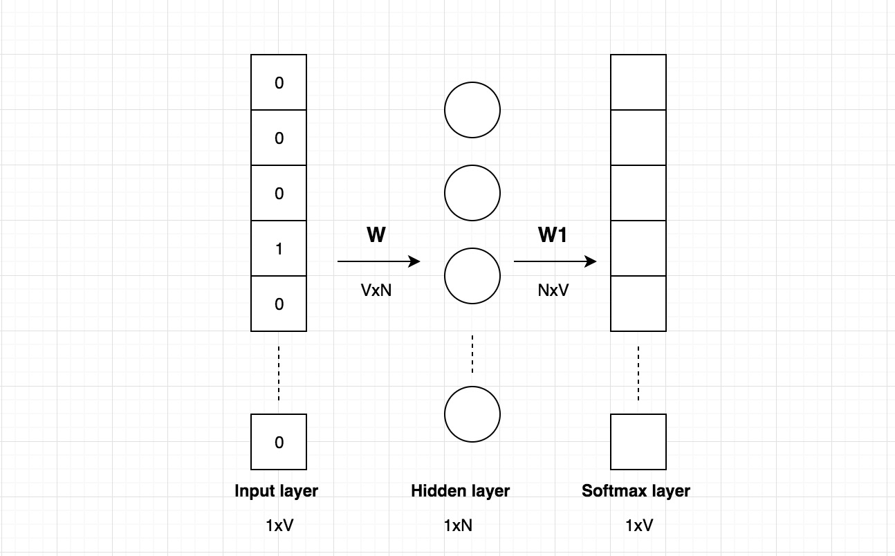
The input is a one-hot vector with a dimension 1xV. The dimension of the weight matrix of the hidden layer is VxN. If we multiply them, we will get a vector with a dimension 1xN.
If you really look at the above matrix calculation, you can see that the weight matrix of the hidden layer actually works as a lookup table, it will effectively just select the matrix row corresponding to the “1”. The output of the matrix calculation is the word embedding/vector for the input word. There are V rows in the weight matrix, each row corresponding to one word vector in the vocabulary. This is why we are only interested in learning the weight matrix of the hidden layer and we call it the word embeddings.
The output layer is a softmax layer with a dimension 1xV, with each element corresponding to the probability that this word is the word that you randomly select nearby the input word.
CBOW
Continuous Bag-of-Words model (CBOW) is just the opposite of Skip-Gram.
For the CBOW model, the task of the simple neural network is: Given a context of words (surrounding a word) in a sentence, the network will predict how likely it is for each word in the vocabulary being the word.
Modifications to the basic model
In reality, it is possible to train the simple neural network and learn the word embeddings. In practice, however, it is infeasible to train the basin Word2Vec model (either Skip-Gram or CBOW) due to the large weight matrix. For example, assume our vocabulary size is 10,000 and the size of the hidden layer is 300, then the hidden layer weight matrix W will have 10000x300=3 million weights. Similarly, the output layer weight matrix W1 will also have 3 million weights.
The training process for such a large neural network will be slow and is prone to overfitting (because of the large number of weights). In the second of their work, the authors of Word2Vec provided some modificaitons to the original model. Three of the most innovative improvements are described below:
Word pairs/Phrases are learnt to reduce the vocabulary size. They presented phrase detection approach to detect phrases like “Los Angeles” and “Golden Globe” and treat them as a single word.
Subsampling frequent words is introduced to diminish the impact of frequent words on the model accuracy. For example, words like “the” and “a” appear a lot across documents and helps little for the creation of a good word embedding.
Negative sampling is a technique to have each training sample only modify a small portion of the weights, rather than all of them. In the basic model, each training example will update all the millions of weights. With negative sampling, we are instead going to randomly select just a small number of “negative” words (let’s say 5) to update the weights for. (In this context, a “negative” word is one for which we want the network to output a 0 for). We will also still update the weights for our “positive” word (the word for which we want the network to output a 1). In this setting, negative sampling will help us reduce the size of the output layer weight matrix from 3 million to 300x6=1,800, which is a huge reduction. In the hidden layer, only the weights for the input word are updated.
All the three modifications above help Word2Vec learn word embeddings fast and achieve good results in the meantime.
Doc2Vec
The concept of Doc2Vec is actually quite simple, if you are already familiar with the Word2vec model. Doc2vec model is based on Word2Vec, with only adding another vector (paragraph ID) to the input. The architecture of Doc2Vec model is shown below:
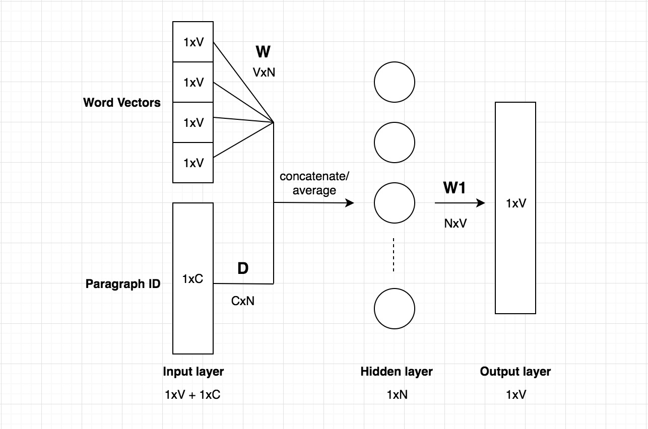
The above diagram is based on the CBOW model, but instead of using just nearby words to predict the word, we also added another feature vector, which is document-unique. So when training the word vectors W, the document vector D is trained as well, and in the end of training, it holds a numeric representation of the document.
The inputs consist of word vectors and document Id vectors. The word vector is a one-hot vector with a dimension 1xV. The document Id vector has a dimension of 1xC, where C is the number of total documents. The dimension of the weight matrix W of the hidden layer is VxN. The dimension of the weight matrix D of the hidden layer is CxN.
The above model is called distributed Memory version of Paragraph Vector (PV-DM). Another Doc2Vec algorithm which is based on Skip-Gram is called Distributed Bag of Words version of Paragraph Vector (PV-DBOW).
Conclusion
Word embeddings are one of the few currently successful applications of unsupervised learning. Pre-trained word embeddings can be used in downstream tasks that use small amounts of labeled data.