Understanding Deep Residual Networks
Deep residual networks (ResNet) took the deep learning world by storm when Microsoft Research released Deep Residual Learning for Image Recognition. These networks led to 1st-place winning entries in all five main tracks of the ImageNet and COCO 2015 competitions, which covered image classification, object detection, and semantic segmentation. The robustness of ResNets has since been proven by various visual recognition tasks and by non-visual tasks involving speech and language. I also used ResNet in addition to other deep learning models in my Phd dissertation research.
This post will summarize the three papers below, which are all written or co-written by ResNet’s inventor Kaiming He, because I believe the original papers give the most intuitive and detailed explanation of the model/networks. Hopefully, this post could help you gain a better understanding of the gist of residual networks.
- Deep Residual Learning for Image Recognition
- Identity mappings in Deep Residual Networks
- Aggregated Residual Transformation for Deep Neural Networks
Intuition on Deep Residual Network (stackoverflow ref)
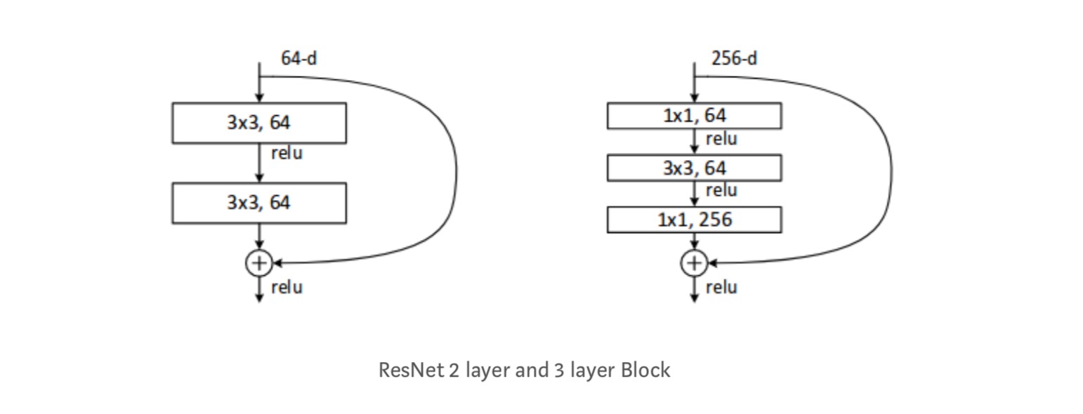
A residual block is displayed as the following:
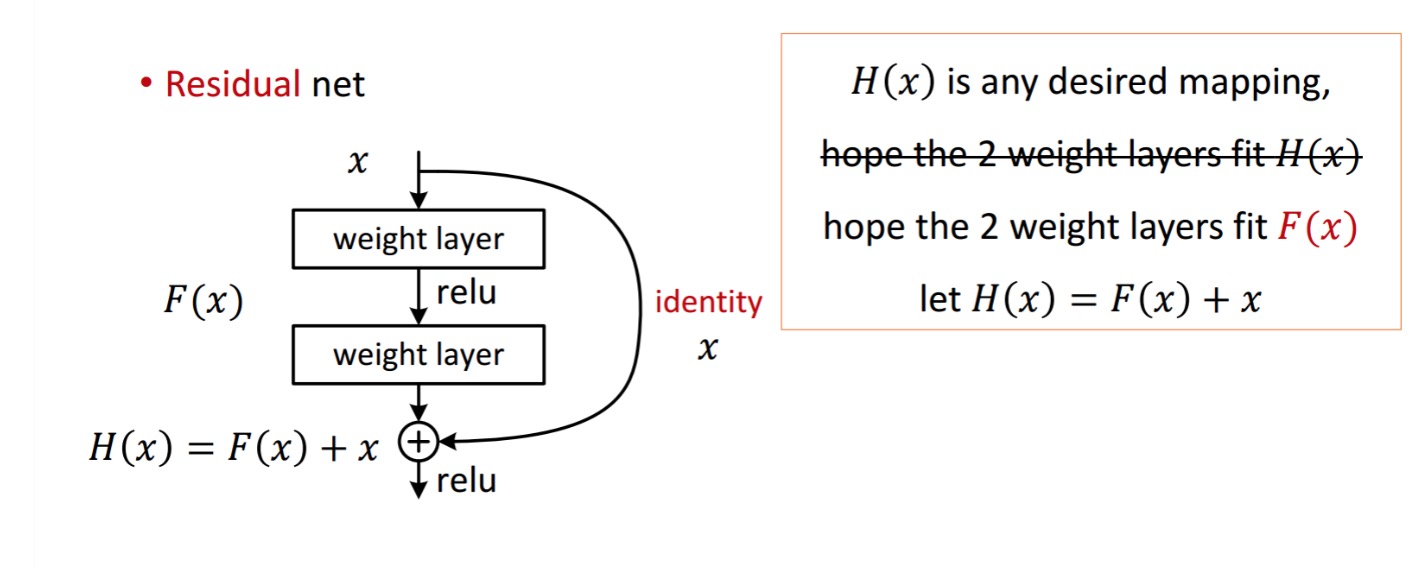
So the residual unit shown obtains \(F(x)\) by processing \(x\) with two weight layers. Then it adds \(x\) to \(F(x)\) to obtain \(H(x)\). Now, assume that \(H(x)\) is your ideal predicted output which matches with your ground truth. Since \(H(x) = F(x) + x\), obtaining the desired \(H(x)\) depends on getting the perfect \(F(x)\). That means the two weight layers in the residual unit should actually be able to produce the desired \(F(x)\), then getting the ideal \(H(x)\) is guaranteed.
\(F(x)\) is obtained from \(x\) as follows.
\[x \rightarrow weight_1 \rightarrow ReLU \rightarrow weight_2\]\(H(x)\) is obtained from \(F(x)\) as follows.
\[F(x) + x \rightarrow ReLU\]The authors hypothesize that the residual mapping (i.e. \(F(x)\)) may be easier to optimize than \(H(x)\). To illustrate with a simple example, assume that the ideal \(H(x) = x\). Then for a direct mapping it would be difficult to learn an identity mapping as there is a stack of non-linear layers as follows.
\[x \rightarrow weight_1 \rightarrow ReLU \rightarrow weight_2 \rightarrow ReLU ... \rightarrow x\]So, to approximate the identity mapping with all these weights and ReLUs in the middle would be difficult.
Now, if we define the desired mapping \(H(x) = F(x) + x\), then we just need get \(F(x) = 0\) as follows.
\[x \rightarrow weight_1 \rightarrow ReLU \rightarrow weight_2 \rightarrow ReLU ... \rightarrow 0\]Achieving the above is easy. Just set any weight to zero and you will get a zero output. Add back \(x\) and you get your desired mapping.
Deep Residual Learning for Image Recognition
Problem
When deeper networks starts converging, a degradation problem has been exposed: with the network depth increasing, accuracy gets saturated and then degrades rapidly.
Seeing Degrading in Action:
Let us take a shallow network and its deeper counterpart by adding more layers to it.
Worst case scenario: Deeper model’s early layers can be replaced with shallow network and the remaining layers can just act as an identity function (Input equal to output).
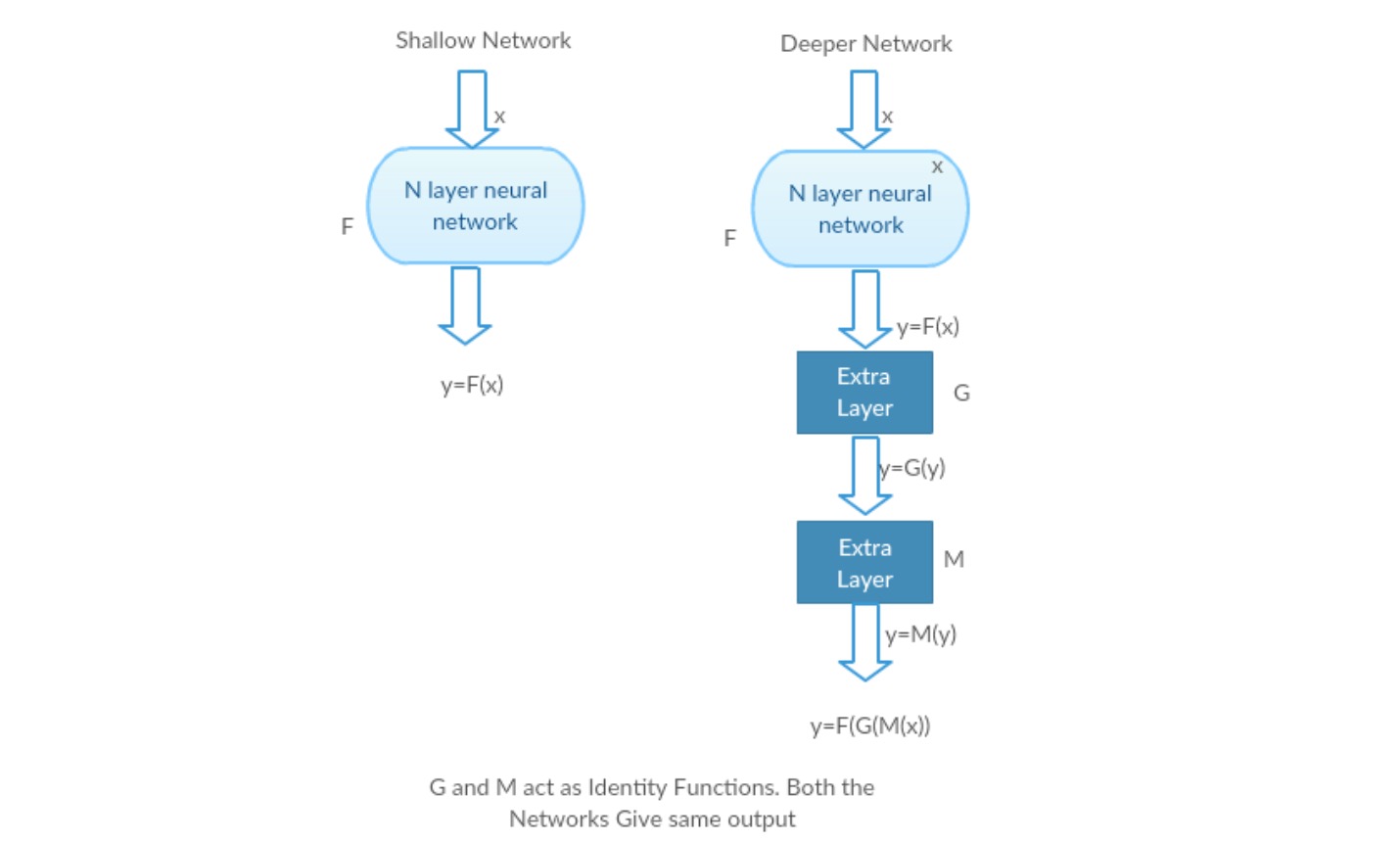
Rewarding scenario: In the deeper network the additional layers better approximates the mapping than it’s shallower counter part and reduces the error by a significant margin.
Experiment: In the worst case scenario, both the shallow network and deeper variant of it should give the same accuracy. In the rewarding scenario case, the deeper model should give better accuracy than it’s shallower counter part. But experiments with our present solvers reveal that deeper models doesn’t perform well. So using deeper networks is degrading the performance of the model. These papers try to solve this problem using Deep Residual learning framework.
How to solve?
Instead of learning a direct mapping of \(x \rightarrow y\) with a function \(H(x)\) (A few stacked non-linear layers). Let us define the residual function using \(F(x) = H(x)-x\), which can be reframed into \(H(x) = F(x)+x\), where \(F(x)\) and \(x\) represents the stacked non-linear layers and the identity function(input=output) respectively.
The author’s hypothesis is that it is easy to optimize the residual mapping function \(F(x)\) than to optimize the original, unreferenced mapping \(H(x)\).
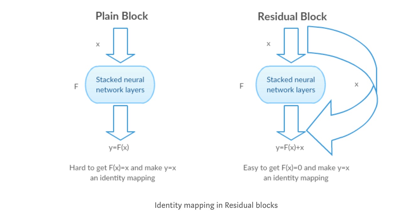
Intuition behind Residual blocks:
Let’s take the identity mapping as an example (e.g. \(H(x)=x\)). If the identity mapping is optimal, we can easily push the residuals to zero (\(F(x) = 0\)) than to fit an identity mapping (\(H(x)=x\)) by a stack of non-linear layers. In simple language it is very easy to come up with a solution like \(F(x)=0\) rather than \(F(x)=x\) using stack of non-linear cnn layers as function (Think about it). So, this function \(F(x)\) is what the authors called Residual function.
The authors made several tests to test their hypothesis. Lets look at each of them now.
Test cases:
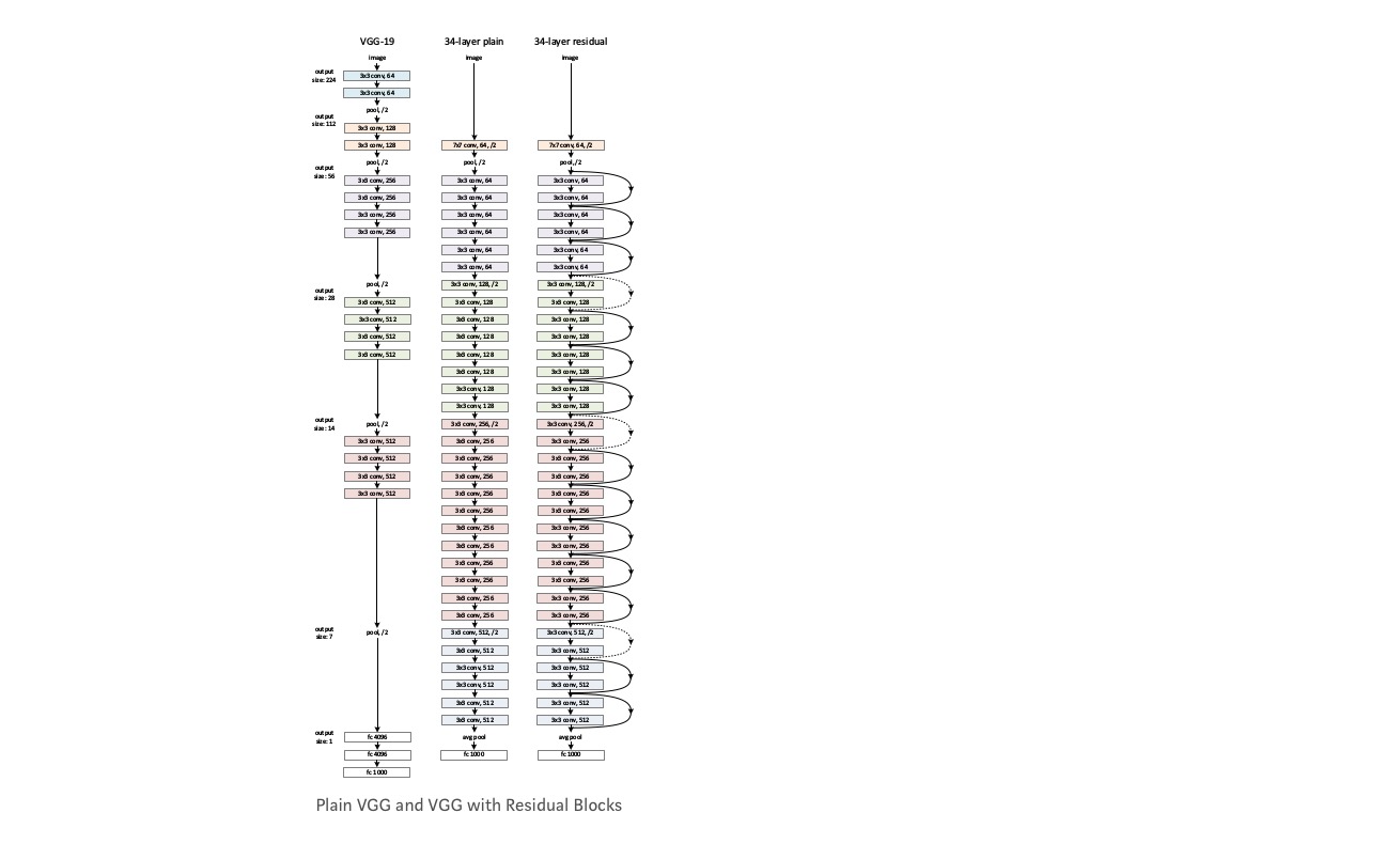
Take a plain network (VGG kind 18 layer network) (Network-1) and a deeper variant of it (34-layer, Network-2) and add Residual layers to the Network-2 (34 layer with residual connections, Network-3).
Designing the network:
- Use 3*3 filters mostly.
- Down sampling with CNN layers with stride 2.
- Global average pooling layer and a 1000-way fully-connected layer with Softmax in the end.
There are two kinds of residual connections:
I. The identity shortcuts (\(x\)) can be directly used when the input (\(x\)) and output (\(F(x)\)) are of the same dimensions.
\[y = F(x, {W_i})+x\]II. When the dimensions change, A) The shortcut still performs identity mapping, with extra zero entries padded with the increased dimension. B) The projection shortcut is used to match the dimension (done by 1*1 conv) using the following formula
\[y = F(x, {W_i})+W_s x\]Results
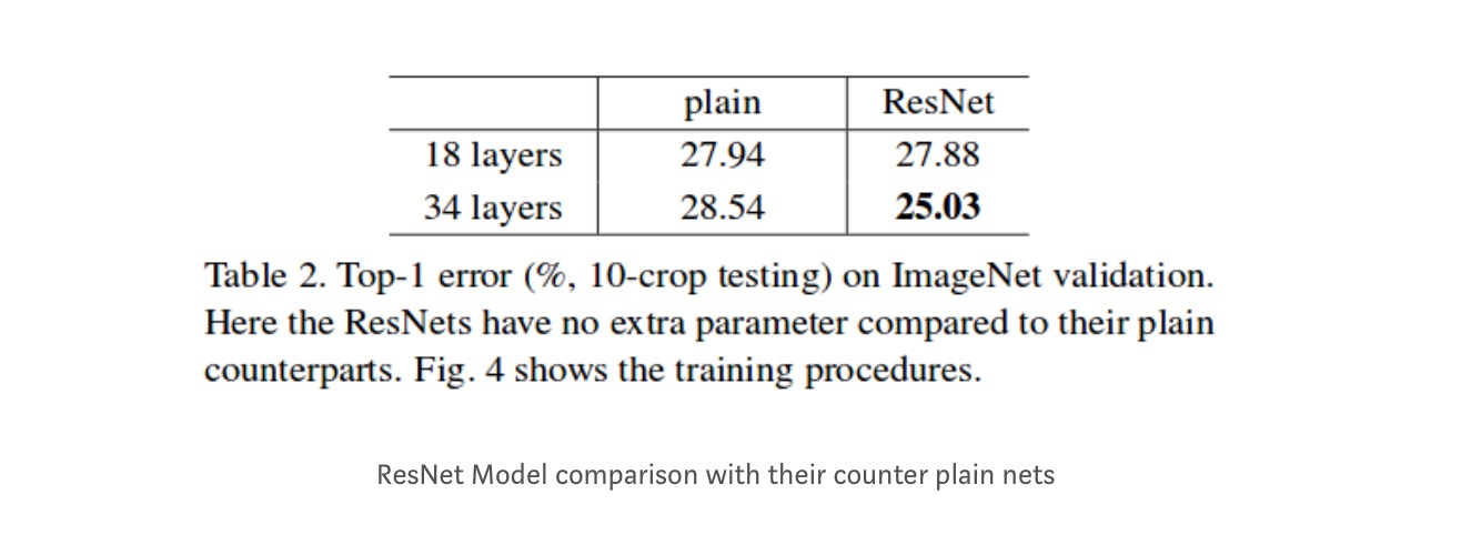
Even though the 18 layer network is just the subspace in 34 layer network, it still performs better. ResNet outperforms by a significant margin in case the network is deeper
Deeper studies
Moreover, more networks are studied:
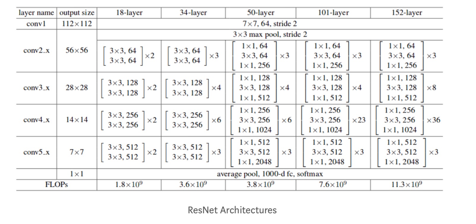
Each ResNet block is either 2 layer deep (Used in small networks like ResNet 18, 34) or 3 layer deep( ResNet 50, 101, 152).
Observations
- ResNet Network Converges faster compared to plain counter part of it.
- Identity vs Projection shorcuts. Very small incremental gains using projection shortcuts (Equation-2) in all the layers. So all ResNet blocks use only Identity shortcuts with Projections shortcuts used only when the dimensions changes.
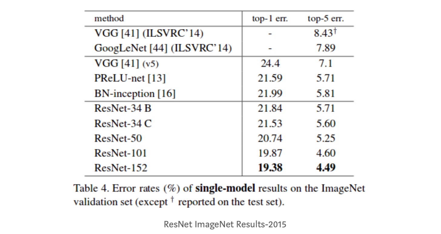
- ResNet-34 achieved a top-5 validation error of 5.71% better than BN-inception and VGG. ResNet-152 achieves a top-5 validation error of 4.49%. An ensemble of 6 models with different depths achieves a top-5 validation error of 3.57%. Winning the 1st place in ILSVRC-2015
Identity mappings in Deep Residual Networks
This paper gives the theoretical understanding of why vanishing gradient problem is not present in Residual networks and the role of skip connections (skip connections mean the input \(x\) or \(h(x)\)) by replacing Identity mapping (x) with different functions.
Introduction
Deep residual networks consist of many stacked “Residual Units”. Each unit can be expressed in a general form:
\[y_l = h(x_l) + F(x_l, W_l) \\ x_{l+1} = f(y_l)\]where \(x_l\) and \(x_{l+1}\) are input and output of the \(l-th\) unit, and \(F\) is a residual function. In the last paper, \(h(x_l)=x_l\) is an identity mapping and \(f\) is a ReLU function.
The central idea of ResNets is to learn the additive residual function \(F\) with respect to \(h(x_l)\), with a key choice of using an identity mapping \(h(x_l)=x_l\). This is realized by attaching an identity skip connection (“shortcut”).
In this paper, we analyze deep residual networks by focusing on creating a “direct” path for propagating information — not only within a residual unit, but through the entire network. Our derivations reveal that if both \(h(x_l)\) and \(f(y_l)\) are identity mappings, the signal could be directly propagated from one unit to any other units, in both forward and backward passes. Our experiments empirically show that training in general becomes easier when the architecture is closer to the above two conditions.
To understand the role of skip connections, we analyze and compare various types of \(h(x_l)\). We find that the identity mapping \(h(x_l)=x_l\) chosen in the last paper achieves the fastest error reduction and lowest training loss among all variants we investigated, whereas skip connections of scaling, gating , and 1×1 convolutions all lead to higher training loss and error. These experiments suggest that keeping a “clean” information path is helpful for easing optimization.
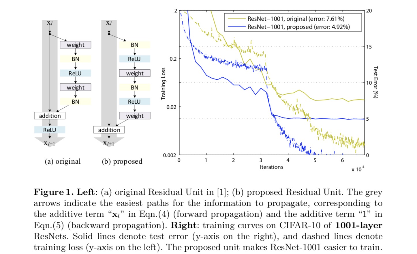
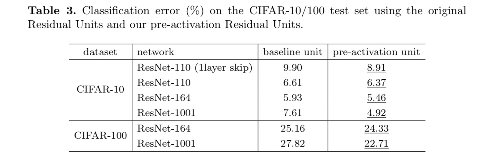
To construct an identity mapping \(f(y_l)=y_l\), we view the activation functions (ReLU and BN) as “pre-activation” of the weight layers, in contrast to conventional wisdom of “post-activation”. This point of view leads to a new residual unit design, shown in the following figure. Based on this unit, we present competitive results on CIFAR-10/100 with a 1001-layer ResNet, which is much easier to train and generalizes better than the original ResNet. We further report improved results on ImageNet using a 200-layer ResNet, for which the counterpart of the last paper starts to overfit. These results suggest that there is much room to exploit the dimension of network depth, a key to the success of modern deep learning.
Analysis of Deep Residual networks
The ResNets developed in the last paper are modularized architectures that stack building blocks of the same connecting shape. In this paper we call these blocks “Residual Units”. The original Residual Unit in the last paper performs the following computation:
\[y_l = h(x_l) + F(x_l, W_l) \\ x_{l+1} = f(y_l)\]Here \(x_l\) is the input feature to the \(l\)-th Residual Unit. \(W_l={W_{l,k}\vert_{1 \le k \le K}}\) is a set of weights (and biases) associated with the \(l\)-th Residual Unit, and \(K\)is the number of layers in a Residual Unit (\(K\) is 2 or 3 in the last paper). \(F\) denotes the residual function, e.g., a stack of two 3×3 convolutional layers in the last paper. The function \(f\) is the operation after element-wise addition, and in the last paper \(f\) is ReLU. The function \(h\) is set as an identity mapping: \(h(x_l)=x_l\).
If \(f\) is also an identity mapping: \(x_{l+1}=y_l\), we can obtain:
\[x_{l+1} = x_l + F(x_l, W_l)\]Recursively we will have:
\[x_L = x_l + \sum_{i=l}^{L-1}{F(x_i,W_i)}\]for any deeper unit \(L\) and any shallower unit \(l\). This equation exhibits some nice properties. (1) The feature \(x_L\) of any deeper unit \(L\) can be represented as the feature \(x_l\) of any shallower unit \(l\) plus a residual function in a form of \(\sum_{i=l}^{L-1}{F}\), indicating that the model is in a residual fashion between any units \(L\) and \(l\). (2) The feature \(x_L = x_0 + \sum_{i=0}^{L-1}{F(x_i,W_i)}\), of any deep unit \(L\), is the summation of the outputs of all preceding residual functions (plus \(x_0\)). This is in contrast to a “plain network” where a feature \(x_L\) is a series of matrix-vector products, say, \(\prod_{i=1}^{L-1}{W_ix_0}\) (ignoring BN and ReLU).
The above equation also leads to nice backward propagation properties. Denoting the loss function as \(E\), from the chain rule of backpropagation we have:
\[\frac{\delta E}{\delta x_l} = \frac{\delta E}{\delta x_L} \frac{\delta x_L}{\delta x_l} = \frac{\delta E}{\delta x_L}(1+\frac{\delta}{\delta x_l}\sum_{i=l}^{L-1}{F(x_i,W_i)})\]The above equation indicates that the gradient \(\frac{\delta E}{\delta x_l}\) can be decomposed into two additive terms: a term of \(\frac{\delta E}{\delta x_L}\) that propagates information directly without concerning any weight layers, and another term of \(\frac{\delta E}{\delta x_L}(\frac{\delta}{\delta x_l}\sum_{i=l}^{L-1}{F(x_i,W_i)})\) that propagates through the weight layers. The additive term of \(\frac{\delta}{\delta x_L}\) ensures that information is directly propagated back to any shallower unit l. The above equation also suggests that it is unlikely for the gradient \(\frac{\delta E}{\delta x_l}\) to be canceled out for a mini-batch, because in general the term \(\frac{\delta}{\delta x_l}\sum_{i=l}^{L-1}{F(x_i,W_i)}\) cannot always be -1 for all samples in a mini-batch. This implies that the gradient of a layer does not vanish even when the weights are arbitrarily small.
The above two equations suggest that the signal can be directly propagated from any unit to another, both forward and backward. The foundation of the first above two equations is two identity mappings: (1) the identity skip connection \(h(x_l)=x_l\), and (2) the condition that \(f\) is an identity mapping.
Importance of identity skip connections
Let’s consider a simple modification, \(h(x_l)=\lambda_l x_l\), to break the identity shortcut:
\[x_{l+1} = \lambda_l x_l + F(x_l, W_l)\]where \(\lambda_l\) is a modulating scalar (for simplicity we still assume \(f\) is identity). Recursively applying this formulation we obtain an equation similar to the above one:
\[x_L = (\prod_{i=l}^{L-1}{\lambda_i})x_l + \sum_{i=l}^{L-1}{\hat{F}(x_i,W_i)}\]where the notation \(\hat{F}\) absorbs the scalars into the residual functions. Similarly, we have backpropagation of the following form:
\[\frac{\delta E}{\delta x_l} = \frac{\delta E}{\delta x_L} \frac{\delta x_L}{\delta x_l} = \frac{\delta E}{\delta x_L}((\prod_{i=l}^{L-1}{\lambda_i})+\frac{\delta}{\delta x_l}\sum_{i=l}^{L-1}{F(x_i,W_i)})\]Unlike the previous equation, in this equation the first additive term is modulated by a factor \(\prod_{i=l}^{L-1}{\lambda_i}\). For an extremely deep network (\(L\) is large), if \(\lambda_i > 1\) for all \(i\), this factor can be exponentially large; if \(\lambda_i < 1\) for all \(i\), this factor can be exponentially small and vanish, which blocks the backpropagated signal from the shortcut and forces it to flow through the weight layers. This results in optimization difficulties as we show by experiments.
In the above analysis, the original identity skip connection is replaced with a simple scaling \(h(x_l)=\lambda_l x_l\). If the skip connection \(h(x_l)\) represents more complicated transforms (such as gating and 1×1 convolutions), in the above equation the first term becomes \(\prod_{i=l}^{L-1}{h_i'}\) where \(h'\) is the derivative of \(h\). This product may also impede information propagation and hamper the training procedure as witnessed in the following experiments.
Experiments on Skip Connections
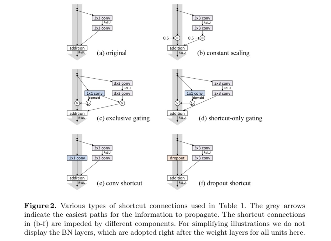
We experiment with the 110-layer ResNet on CIFAR-10. This extremely deep ResNet-110 has 54 two-layer Residual Units (consisting of 3×3 convolutional layers) and is challenging for optimization. Various types of skip connections are experimented. See the following figure:
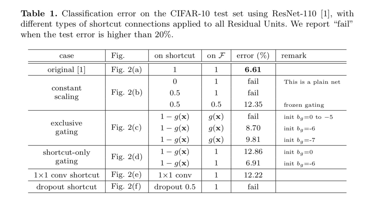
The classification results are displayed in the following table:
As indicated by the grey arrows in the above figure, the shortcut connections are the most direct paths for the information to propagate. Multiplicative manipulations (scaling, gating, 1×1 convolutions, and dropout) on the shortcuts can hamper information propagation and lead to optimization problems.
It is noteworthy that the gating and 1×1 convolutional shortcuts introduce more parameters, and should have stronger representational abilities than identity shortcuts. In fact, the shortcut-only gating and 1×1 convolution cover the solution space of identity shortcuts (i.e., they could be optimized as identity shortcuts). However, their training error is higher than that of identity shortcuts, indicating that the degradation of these models is caused by optimization issues, instead of representational abilities.
Usage of Activation Functions
Experiments in the above section are under the assumption that the after-addition activation \(f\) is the identity mapping. But in the above experiments \(f\) is ReLU as designed in the first paper. Next we investigate the impact of \(f\).
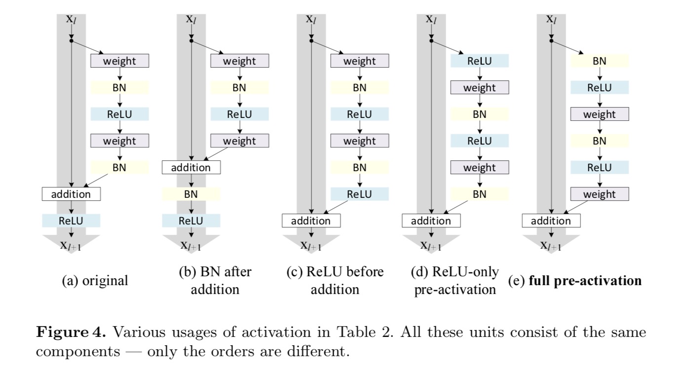
We want to make \(f\) an identity mapping, which is done by re-arranging the activation functions (ReLU and/or BN, batch normalization). In the following figure, the original Residual Unit in the last paper has a shape in Fig. 4(a) – BN is used after each weight layer, and ReLU is adopted after BN except that the last ReLU in a Residual Unit is after elementwise addition (\(f\) = ReLU). Fig. 4(b-e) show the alternatives we investigated.
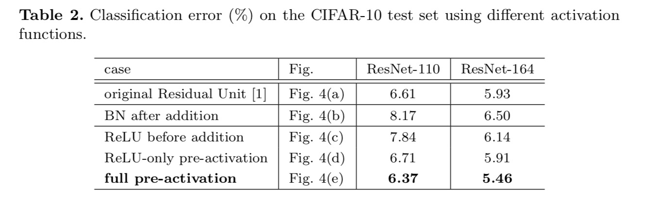
Experiments on Activation
In this section we experiment with ResNet-110 and a 164-layer Bottleneck architecture (denoted as ResNet-164). A bottleneck Residual Unit consist of a 1×1 layer for reducing dimension, a 3×3 layer, and a 1×1 layer for restoring dimension. As designed in the last paper, its computational complexity is similar to the two-3×3 Residual Unit.
Post-activation or pre-activation?
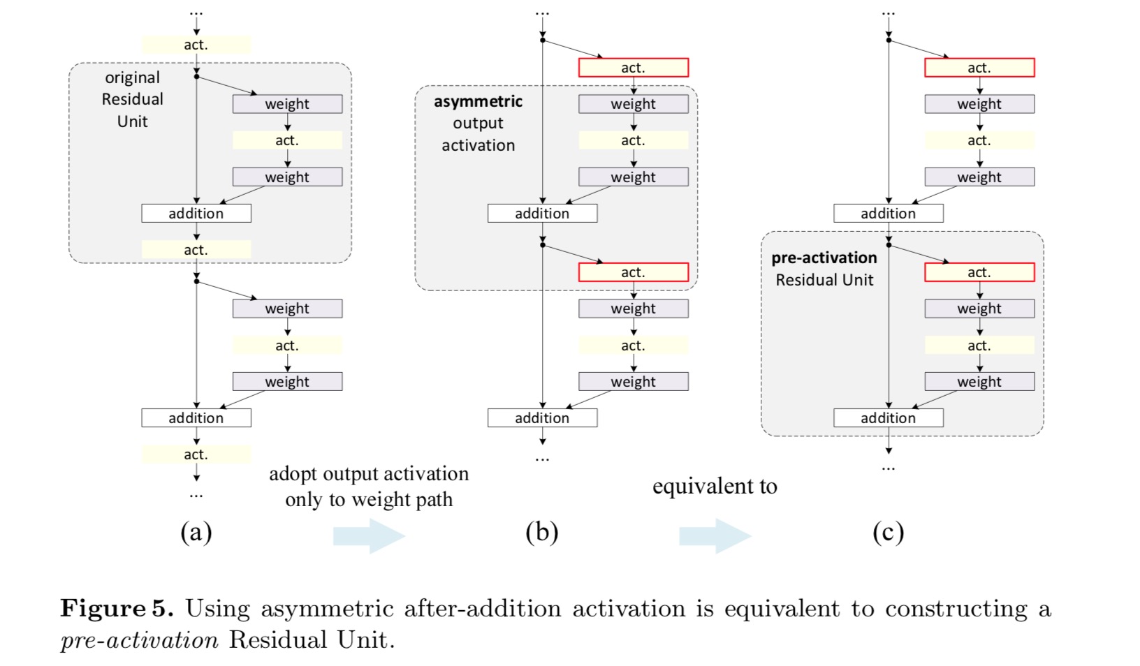
In the original design, the activation \(x_{l+1} = f(y_l)\) affects both paths in the next Residual Unit: \(y_{l+1} = f(y_l) + F(f(y_l), W_{l+1})\). Next we develop an asymmetric form where an activation \(\hat{f}\) only affects the \(F\) path: \(y_{l+1} = y_l + F(\hat{f}(y_l), W_{l+1})\), for any \(l\). By renaming the notations, we have the following form:
\[x_{l+1} = x_l + F(\hat{f}(x_l), W_{l})\]For this new Residual Unit as in the above equation, the new after-addition activation becomes an identity mapping. This design means that if a new after-addition activation \(\hat{f}\) is asymmetrically adopted, it is equivalent to recasting \(\hat{f}\) as the pre-activation of the next Residual Unit. This is illustrated in the following figure:
The distinction between post-activation/pre-activation is caused by the presence of the element-wise addition. For a plain network that has N layers, there are N − 1 activations (BN/ReLU), and it does not matter whether we think of them as post- or pre-activations. But for branched layers merged by addition, the position of activation matters. The Various usages of activation are displayed in Figure 4.
We experiment with two such designs: (1) ReLU-only pre-activation and (2) full pre-activation where BN and ReLU are both adopted before weight layers. Somehow surprisingly, when BN and ReLU are both used as pre-activation, the results are improved by healthy margins
We find the impact of pre-activation is twofold. First, the optimization is further eased (comparing with the baseline ResNet) because f is an identity mapping. Second, using BN as pre-activation improves regularization of the models.
Conclusion
This paper investigates the propagation formulations behind the connection mechanisms of deep residual networks. Our derivations imply that identity short- cut connections and identity after-addition activation are essential for making information propagation smooth. Ablation experiments demonstrate phenom- ena that are consistent with our derivations. We also present 1000-layer deep networks that can be easily trained and achieve improved accuracy.
Aggregated Residual Transformation for Deep Neural Networks
Introduction
Research on visual recognition is undergoing a transition from “feature engineering” to “network engineering”. Human effort has been shifted to designing better network architectures for learning representations.
Designing architectures becomes increasingly difficult with the growing number of hyper-parameters especially when there are many layers. The VGG-nets exhibit a simple yet effective strategy of constructing very deep networks: stacking building blocks of the same shape. This strategy is inherited by ResNets which stack modules of the same topology. This simple rule reduces the free choices of hyper parameters, and depth is exposed as an essential dimension in neural networks. Moreover, we argue that the simplicity of this rule may reduce the risk of over-adapting the hyperparameters to a specific dataset. The robustness of VGG-nets and ResNets has been proven by various visual recognition tasks and by non-visual tasks involving speech and language.
Unlike VGG-nets, the family of Inception models have demonstrated that carefully designed topologies are able to achieve compelling accuracy with low theoretical complexity. The Inception models have evolved over time, but an important common property is a split-transform-merge strategy. In an Inception module, the input is split into a few lower-dimensional embeddings (by 1×1 convolutions), transformed by a set of specialized filters (3×3, 5×5, etc.), and merged by concatenation. The split-transform-merge behavior of Inception modules is expected to approach the representational power of large and dense layers, but at a considerably lower computational complexity.
Despite good accuracy, the realization of Inception models has been accompanied with a series of complicating factors. Although careful combinations of these components yield excellent neural network recipes, it is in general unclear how to adapt the Inception architectures to new datasets/tasks, especially when there are many factors and hyper-parameters to be designed.
In this paper, we present a simple architecture which adopts VGG/ResNets’ strategy of repeating layers, while exploiting the split-transform-merge strategy in an easy, extensible way. A module in our network performs a set of transformations, each on a low-dimensional embedding, whose outputs are aggregated by summation. We pursuit a simple realization of this idea — the transformations to be aggregated are all of the same topology. This design allows us to extend to any large number of transformations without specialized designs.
We empirically demonstrate that our aggregated transformations outperform the original ResNet module, even under the restricted condition of maintaining computational complexity and model size. We emphasize that while it is relatively easy to increase accuracy by increasing capacity (going deeper or wider), methods that increase accuracy while maintaining (or reducing) complexity are rare in the literature.
Our method indicates that cardinality (the size of the set of transformations) is a concrete, measurable dimension that is of central importance, in addition to the dimensions of width and depth. Experiments demonstrate that increasing cardinality is a more effective way of gaining accuracy than going deeper or wider, especially when depth and width starts to give diminishing returns for existing models.
Our neural networks, named ResNeXt (suggesting the next dimension), outperform ResNet-101/152, ResNet-200, Inception-v3, and Inception-ResNet-v2 on the ImageNet classification dataset. In particular, a 101-layer ResNeXt is able to achieve better accuracy than ResNet-200 but has only 50% complexity. Moreover, ResNeXt exhibits considerably simpler designs than all Inception models.
Method
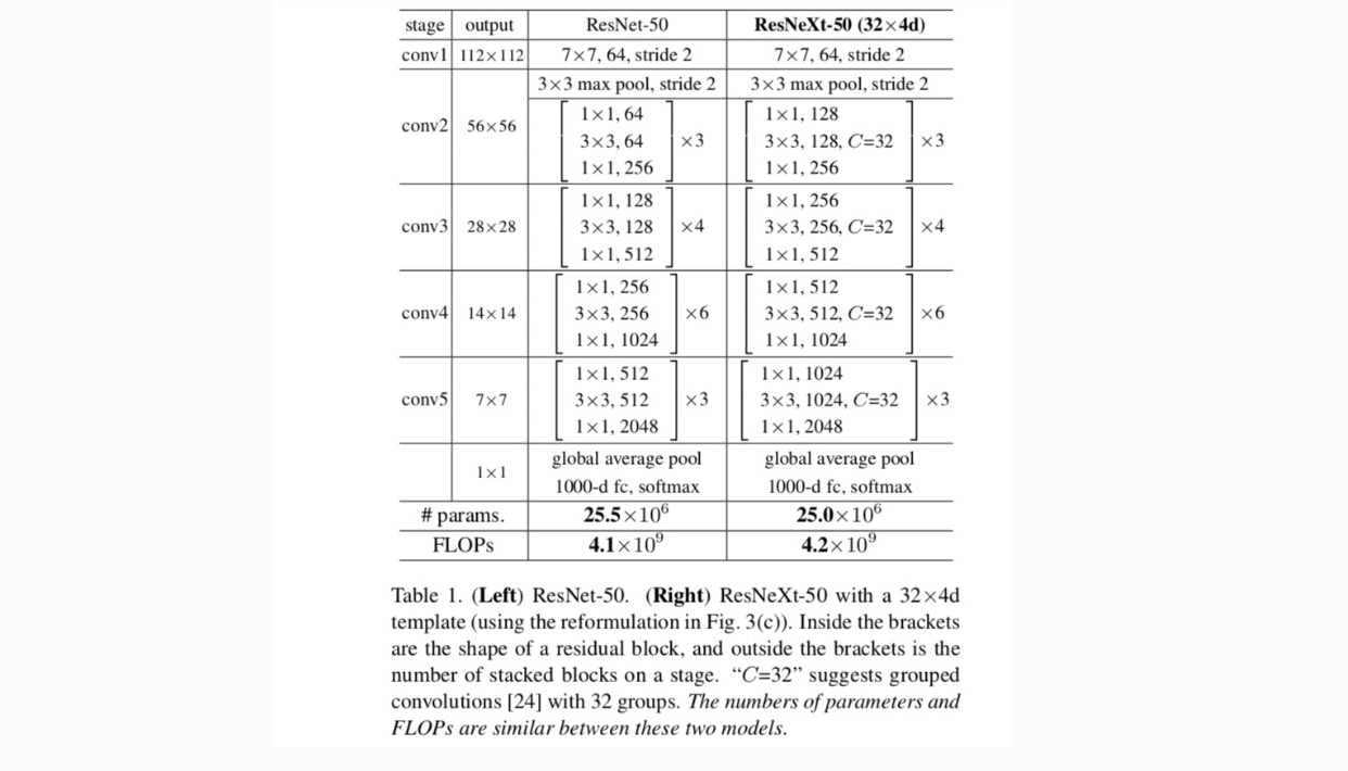
We adopt a highly modularized design following VGG/ResNets. Our network consists of a stack of residual blocks. These blocks have the same topology, and are subject to two simple rules inspired by VGG/ResNets: (1) if producing spatial maps of the same size, the blocks share the same hyper-parameters (width and filter sizes), and (2) each time when the spatial map is downsampled by a factor of 2, the width of the blocks is multiplied by a factor of 2. The second rule ensures that the computational complexity, in terms of FLOPs (floating-point operations, in #of multiply-adds), is roughly the same for all blocks.
With these two rules, we only need to design a template module, and all modules in a network can be determined accordingly. So these two rules greatly narrow down the design space and allow us to focus on a few key factors. The networks constructed by these rules are in Table 1.
The simplest neurons in artificial neural networks perform inner product (weighted sum), which is the elementary transformation done by fully-connected and convolutional layers.
\[\sum_{i=1}^D{w_ix_i}\]The above operation can be recast as a combination of splitting, transforming, and aggregating. (1): Splitting: the vector \(X\) is sliced as a low-dimensional embedding, and in the above, it is a single-dimension subspace \(x_i\) (2) Transforming: the low-dimensional representation is transformed, and in the above, it is simply scaled: \(w_ix_i\) (3) Aggregating: the transformations in all embeddings are aggregated by \(\sum{i=1}^D\).
Given the above analysis of a simple neuron, we consider replacing the elementary transformation (w_i, x_i) with a more generic function, which in itself can also be a network. Formally, we present aggregated transformations as:
\[F(X) = \sum_{i=1}^C{T_i(X)}\]where \(T_i(X)\) can be an arbitrary function. Analogous to a simple neuron, \(T_i\) should project \(X\) into an (optionally low-dimensional) embedding and then transform it.
We refer to \(C\) as cardinality. \(C\) is in a position similar to \(D\) in \(\sum_{i=1}^D{w_ix_i}\), but \(C\) need not equal \(D\) and can be an arbitrary number. We show by experiments that cardinality is an essential dimension and can be more effective than the dimensions of width and depth.
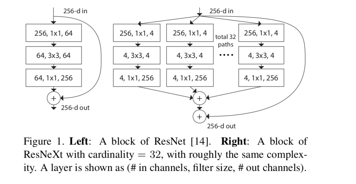
In this paper, we consider a simple way of designing the transformation functions: all \(T_i\)’s have the same topology. This extends the VGG-style strategy of repeating layers of the same shape. We set the individual transformation \(T_i\) to be the bottleneck-shaped architecture illustrated in Fig. 1 (right). In this case, the first 1×1 layer in each \(T_i\) produces the low-dimensional embedding.
The aggregated transformation in last equation serves as the residual function:
\[y = X + \sum_{i=1}^C{T_i(X)}\]where \(y\) is the output.
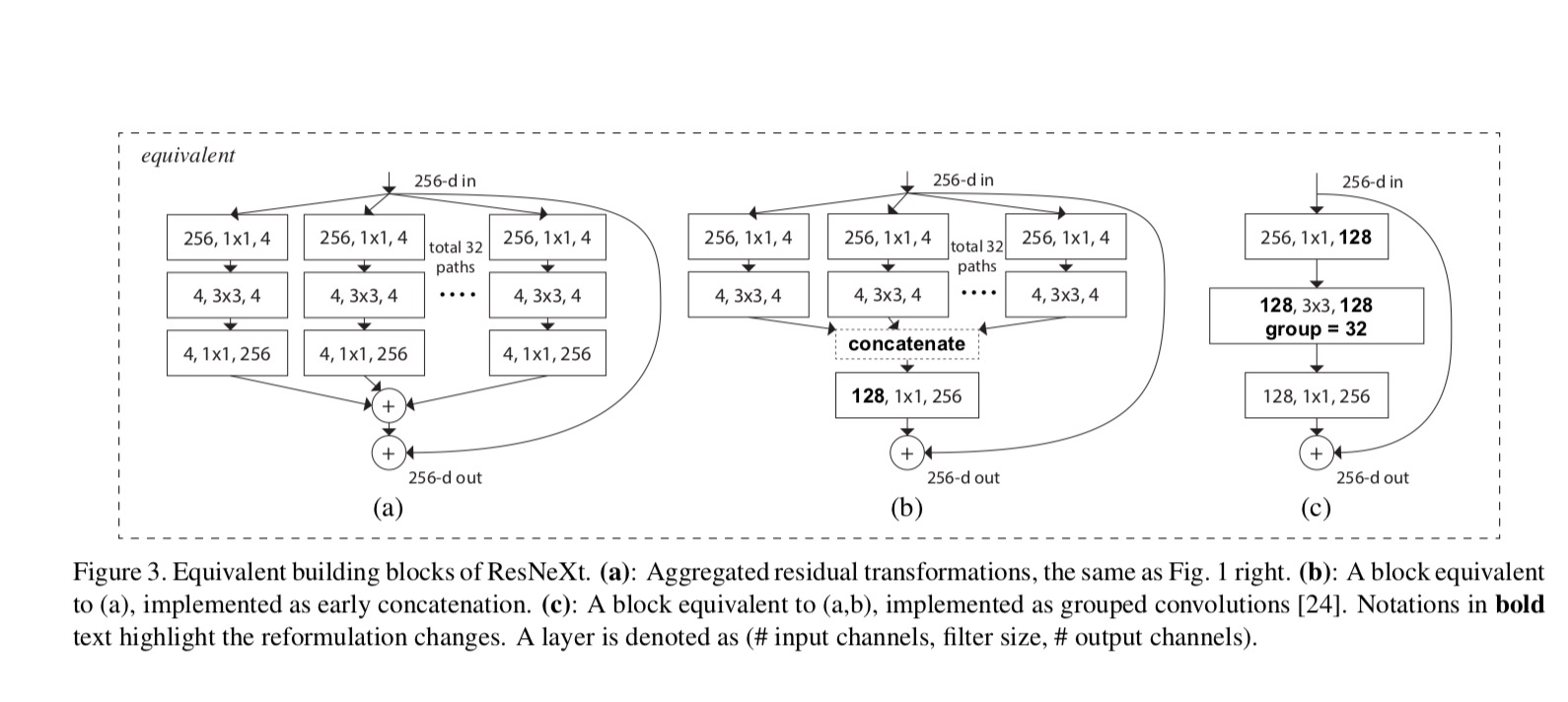
The relationships between ResNeXt and Inception-ResNet/Grouped-Convolutions are shown in the following figure:
When we evaluate different cardinalities \(C\) while preserving complexity, we want to minimize the modification of other hyper-parameters. We choose to adjust the width of the bottleneck (e.g., 4-d in Fig 1(right)), because it can be isolated from the input and output of the block. This strategy introduces no change to other hyper-parameters (depth or input/output width of blocks), so is helpful for us to focus on the impact of cardinality.
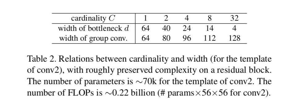
In Fig. 1(left), the original ResNet bottleneck block has \(256\cdot 64+3\cdot 3\cdot 64\cdot 64+64\cdot 256 \approx 70k\) parameters and proportional FLOPs (on the same feature map size). With bottleneck width \(d\), our template in Fig. 1(right) has: \(C\cdot (256\cdot d + 3\cdot 3\cdot d\cdot d + d\cdot 256)\) parameters and proportional FLOPs. When \(C = 32\) and \(d = 4\), this number \(\approx 70k\). The following table shows the relationship between cardinality \(C\) and bottleneck width \(d\).
Experiments
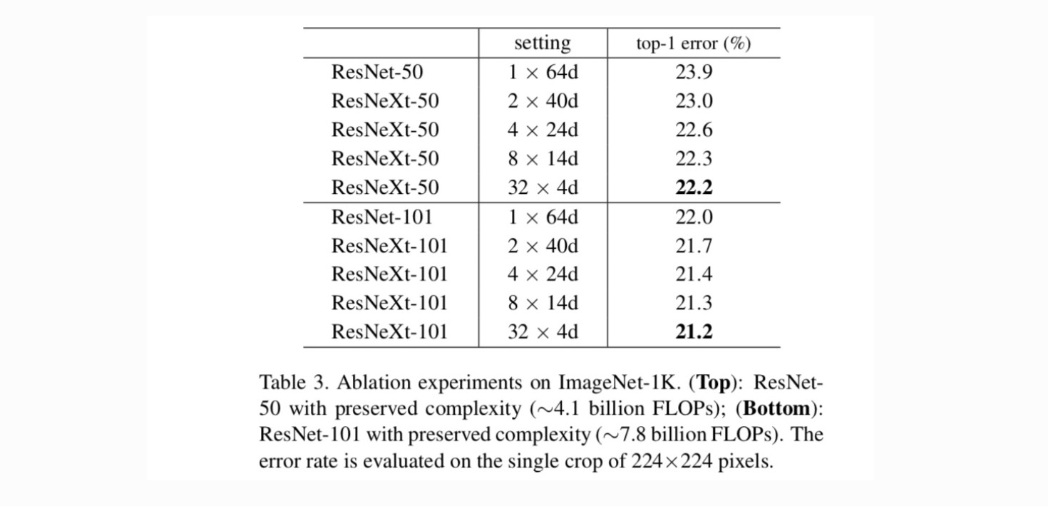
Cardinality vs. Width. We first evaluate the trade-off between cardinality \(C\) and bottleneck width, under preserved complexity as listed in Table 2. Table 3 shows the results. Comparing with ResNet-50, the 32×4d ResNeXt-50 has a validation error of 22.2%, which is 1.7% lower than the ResNet baseline’s 23.9%. With cardinality \(C\) increasing from 1 to 32 while keeping complexity, the error rate keeps reducing. Furthermore, the 32×4d ResNeXt also has a much lower training error than the ResNet countetpart, suggesting that the gains are not from regularization but from stronger representations.
Increasing Cardinality vs. Deeper/Wider.
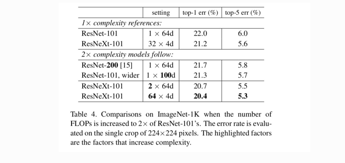
Next we investigate increasing complexity by increasing cardinality C or increasing depth or width. We compare the following variants (1) Going deeper to 200 layers. We adopt the ResNet-200. (2) Going wider by increasing the bottleneck width. (3) Increasing cardinality by doubling C.
Table 4 shows that increasing complexity by 2× consistently reduces error vs. the ResNet-101 baseline (22.0%). But the improvement is small when going deeper (ResNet-200, by 0.3%) or wider (wider ResNet-101, by 0.7%). On the contrary, increasing cardinality C shows much better results than going deeper or wider.
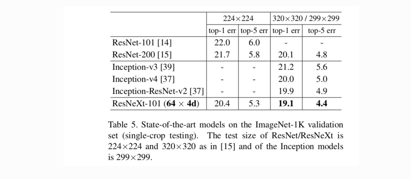
Comparisons with state-of-the-art results. Table 5 shows more results of single-crop testing on the ImageNet validation set. Our results compare favorably with ResNet, Inception-v3/v4, and Inception-ResNet-v2, achieving a single-crop top-5 error rate of 4.4%. In addition, our architecture design is much simpler than all Inception models, and requires considerably fewer hyper-parameters to be set by hand.